
Four Ways to Find a Leak, and What Each One Misses
Visual checks, sensors, tracers and pipework testing each miss something in liquid cooling for data centers. A case-file on detection limits, and why fluid condition is the first line.
Every liquid cooling for data centers deployment ships with leak detection. Ropes under the manifolds, sensors in the trays, a dashboard tile that turns amber. And every year, somewhere, a hall still loses a rack to fluid it did not see coming. The gap is not negligence. It is the nature of detection: every method watches some of the truth and misses the rest. This case file records what each method misses, then turns to the quieter question underneath — whether the leak needed to happen at all. The file is compiled from Glacier Coolant service work on cold-plate loops, where we sit on the chemistry side of exactly this layering.
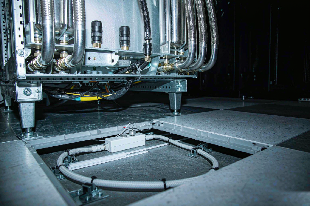
Exhibit one: the visual inspection
The oldest method. An engineer walks the aisle and looks.
| Strength | Limit |
|---|---|
| Finds obvious, external, developed leaks | Depends entirely on experience and lighting |
| Costs nothing to deploy | Blind inside trays, channels and enclosures |
| Catches what sensors miss at first glance | Sees the leak only after it is visible — late by definition |
The file closes exhibit one quickly: visual inspection is a complement, never a system. It confirms what the dashboard suspected and finds what the dashboard ignores, but a leak inside a cable trench or beneath a manifold roof stays invisible until it is a problem.
Exhibit two: point sensors and detection rope
Leak-sensing cable laid along drip paths, spot sensors in trays. The standard equipment of every cold-plate hall, and rightly so — response times are good and coverage is legible on a floor plan.
| Strength | Limit |
|---|---|
| Fast, localizable alarms | Coverage ends where the rope ends |
| Integrates with monitoring platforms | Detection dead zones behind equipment |
| Proven technology, low cost per metre | Sensitive to temperature swings and dust; some sensors miss non-conductive fluids |
The last limit deserves a pause. Detection techniques that rely on conductivity cannot see a non-conductive fluid at all — the sensor stays dry-eyed while a pool grows. That fact matters more as fleets mix chemistries across halls, and it is one reason fluid choice and detection design must be decided together, not by different departments.
Exhibit three: tracer-based leak detection
Add a marker to the fluid, look for the marker where it should not be. Elegant in principle.
| Strength | Limit |
|---|---|
| Finds the fluid, not just the water | Quantifying the leak rate is hard |
| Useful for confirming a suspected path | The marker itself must not contaminate the loop |
| Works where sensors have no reach | Compatibility of the tracer with fluid chemistry and seals must be proven |
The file's verdict: tracers are an investigation tool, not a monitoring system. Deploy them when chasing a suspected weep; do not build a maintenance philosophy on them.
Exhibit four: pipework integrity testing
Pressure decay, helium checks, acoustic methods on welds and joints. Commissioning-grade techniques that find the weakness before the fluid does.
| Strength | Limit |
|---|---|
| Finds defects pre-service | High skill threshold and cost to run fleet-wide |
| Locates potential failure points | Cannot cover everything continuously |
| Best value at build and after repairs | Offline by nature — not a real-time guard |
The pattern across all four exhibits is now visible. Every method is either early-but-incomplete or complete-but-late. No hardware closes that gap, because the gap is physical. This is where the file turns from detection to the other question.
The inversion: prediction from operating data
Modern halls increasingly run inverse-problem diagnostics: instead of watching for fluid where it should not be, the system watches operating data for the signatures a developing failure leaves behind. Three families of method share the work.
| Family | How it works | Where it shines | Where it struggles |
|---|---|---|---|
| Model-based | Compares measured outputs against a physics model's predictions | Explainable; needs few labelled failures | Model fidelity limits sensitivity |
| Rule-based | Matches sensor patterns against expert rules | Transparent; easy to audit | Rules lag novel failure modes |
| Data-driven | Learns failure signatures from history | Handles nonlinear, high-dimensional systems | Starved of failure data; weak explainability |
The data-driven family carries the industry's hopes — and its hardest limit. Real failure samples are scarce and skewed; early weak signatures drown in noise and sensor bias; out-of-distribution failures arrive precisely when the model is least ready. The algorithms are improving every year. None of that improvement matters if the data feeding them is dirty — and the dirtiest input in the system is a drifting, ageing heat transfer fluid. A model learns from what it is shown. Show it a loop whose chemistry wanders, and it learns wander. Show it a stable loop, and every real deviation stands out against a quiet floor.
Why fluid condition is the data baseline
A cold-plate loop's sensors read a system whose chemistry is quietly changing. An ageing coolant shifts viscosity, acidity and heat transfer behaviour. Deposits narrow channels. Local hotspots move operating points. The diagnostic models see all of this as "change", and change is exactly what they must distinguish from failure. A fluid drifting on its own manufactures false signatures and buries true ones.
The conclusion the case file records: diagnosis works on a trustworthy baseline, and the baseline is chemistry. A coolant engineered to stay stable — resisting thermal decomposition and oxidation, holding its corrosion film, staying clean and low-viscous — gives the models a system whose drift means something. That is what we mean by the first line of defence. The degradation failure chain shows how an unstable fluid funds its own failures; the long-term stability blueprint shows how to specify against it.
Glacier Coolant's position in this file is specific: LM-425D-YS, our purpose-built secondary-loop fluid, was formulated so that the operating data a hall collects stays meaningful for years — low, stable starting conductivity; film-forming chemistry on the loop's actual metals; viscosity that does not creep across the band. A stable fluid is what makes the data worth collecting in the first place; the baseline has to be set, not hoped for.
A note on immersion halls
The same two-layer logic holds where the hardware sits submerged. Data center immersion cooling raises different questions — fluid selection dominates even more, and the electrical isolation topic around a dielectric liquid belongs to the immersion spec sheet rather than this file — but the layering is identical: chemistry prevents, detection watches. Halls that skip the first layer pay for it in the second.
The two-line defence, on one page
| Layer | What it does | What it costs |
|---|---|---|
| Line one: stable coolant chemistry | Makes most failures not happen; keeps the data baseline clean | Specification discipline at purchase; monitoring in service |
| Line two: detection and diagnostics | Catches what line one cannot fully prevent | Hardware, sensors, algorithms — all limited by line one's quality |
Three field notes on detection limits
Abstract limits become concrete in field notes. Three patterns recur when we review detection setups alongside fluid records.
The dry-eyed sensor. A hall running mixed chemistries relied on conductive sensors everywhere. Its immersion-adjacent test cell used a fluid the sensors could not see. The dashboard was green while a tray filled. The fix cost one afternoon: map fluid types to sensor types, room by room, and mark the blind pairs in the monitoring legend.
The alarm that trained the team. A temperature-sensitive rope produced false alarms every summer shoulder season. After the third nuisance page, the duty team raised the alarm threshold. The next real weep arrived quietly, under a raised line, and ran for eleven days. Detection systems need seasonal baselines as much as loops need chemical ones — otherwise the humans tune the truth out.
The clean model, the dirty year. A data-driven diagnostic pilot performed well in month one and degraded by month four. No algorithm had changed. The fluid had: make-up discipline slipped, readings drifted, and the model's baseline rotted under it. The pilot's lesson was not about machine learning. It was that a data baseline is perishable, and the fridge it lives in is the fluid specification.
| Field note | Root cause | Lasting fix |
|---|---|---|
| Dry-eyed sensor | Chemistry/sensor mismatch | Fluid-to-sensor mapping per room |
| Trained alarm | Seasonal drift vs fixed threshold | Seasonal baselines and recalibration |
| Dirty year | Perished data baseline | Fluid spec owned as part of the monitoring system |
Each note ends the same way. The detection layer was designed carefully; the chemistry layer was assumed. The gap between the two is where the losses lived.
Two questions settle most budget arguments. How much fluid can leave before anyone notices — not in theory, but given where the sensors actually sit. And how long the loop can run after that point before something electrical happens. Sites that answer both honestly usually find their money belongs in the first layer. Budget conversations usually argue about line two. The ledger lives in line one. Send us your current detection configuration and your latest fluid test record; we will return the gap list between your two lines, and what closing the first-layer gaps would actually take. The product collection is the catalogue, and the LM-425D-YS reading is the natural next exhibit.
FAQ
How are coolant leaks detected in data centers?
Four direct methods: visual inspection, point sensors and detection rope, tracer-based detection, and pipework integrity testing. Each has blind spots, which is why mature halls layer them — and why fluid chemistry remains the first line.
What are the limits of leak detection?
Visual checks see only developed, visible leaks. Sensors stop where the rope stops and can miss non-conductive fluids. Tracers investigate but do not quantify continuously. Pipework testing is skilled, costly and offline. Direct detection as a class struggles with slow, weak, hidden failures.
Can AI predict coolant leaks?
Inverse-problem diagnostics — model-based, rule-based and data-driven — can catch developing failures early. Their effectiveness depends on failure samples and, above all, on a trustworthy data baseline. An ageing, drifting coolant contaminates that baseline with false signatures.
Why does coolant chemistry matter for diagnostics?
Diagnostic models must separate real failure signatures from ordinary drift. A stable coolant makes drift meaningful; a degrading fluid manufactures change that looks like failure and hides failure that looks like change.
What is a detection dead zone?
Any volume the detection hardware cannot watch: behind equipment, inside channels, above cable trays. Dead zones are why halls with full rope coverage still experience unseen leaks.
Do sensors detect all coolant types?
No. Sensors that rely on conductivity miss non-conductive fluids entirely. If your hall runs or plans mixed chemistries, verify detection coverage against each fluid type explicitly.
Is detection useless if chemistry is the first line?
The opposite. Detection is the safety net for what chemistry cannot prevent — mechanical damage, fitting failures, human error. The layering works when line one keeps failure rates low and data clean, and line two catches the residue.
What makes a coolant "stable" in this context?
Documented resistance to thermal decomposition and oxidation, film-forming corrosion protection on the loop's metals, cleanliness against microbial and particulate fouling, and a viscosity profile that does not drift across the operating band.